Alternate Color Between Excel Rows
In Excel, assigning an alternating color scheme to rows is known as color banding. Start by selecting the cells you want to apply color banding too. Or press Ctrl+A to select the entire sheet.
Next, select the Home tab on the Ribbon, select Styles, and click Conditional Formatting.
A drop-down menu will display; click New Rule.
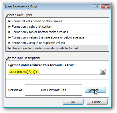
The New Formatting Rule dialog appears. Click the bottom option labeled Use a Formula to Determine Which Cells to Format. In the empty format value field, copy and paste in the following formula: The New Formatting Rule window will look like this. Click Format.
Pick a fill color and click OK.
The New Formatting Rule windows will display the color Preview. Click OK.
The section of your spreadsheet will now be color-banded.
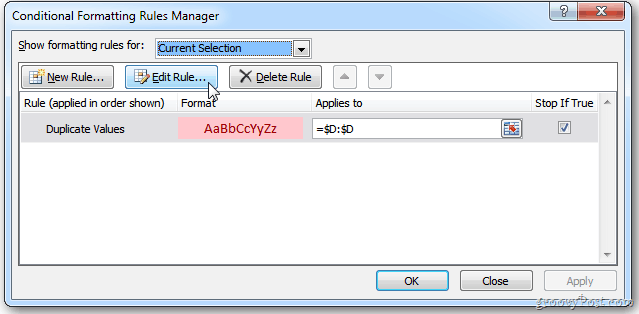
If you want to change the color or add more cells, highlight the cells on the spreadsheet. Then on the Ribbon, go to Conditional Formatting > > Manage Rules.
The Conditional Formatting Rules Manager window comes up. Click Edit Rule.
The Edit Formatting Screen appears and can adjust accordingly.
I question the formula. Use =mod(row()/2)>0. It works equally well and is less convoluted. In the mod formula, the >0 part isn’t necessary. 0 will evaluate to FALSE and any non-zero number will evaluate to TRUE, therefore; =MOD(ROW(),2) will suffice. If you want to start with a blank row, instead of a filled row, just subtract 1 in the formula: =MOD(ROW(),2)-1 Comment Name * Email *
Δ Save my name and email and send me emails as new comments are made to this post.
![]()


